K‑means clustering with SQLMesh Python models

Introduction

SQLMesh is versatile. One core reason is its ability to run SQL, Jinja, and Python models within a single project. Let’s explore this functionality through a marketing use case.

Scenario: Marketing wants to run targeted campaigns based on the projected “lifetime value” of existing customers. Marketing wants to know which of their customers have Top, High, Mid, Low, and Very Low revenue potential. We can answer this question with a k-means clustering algorithm. Raw metrics exist in our pipeline, but implementing segmentation logic is complex or nearly impossible using only SQL. This is where a SQLMesh Python model shines: you keep the same plans, environments, lineage, and promotion flow, but run Python to do what SQL can’t.

In this tutorial, you’ll: 

• Set up the project
• Add a SQL model that calculates lifetime value
• Add a Python model that clusters customers using k‑means
• Plan in a dev environment
• Preview and validate results
• Promote to prod
• Add tests and review output

Why Use a Python Model?

Python models are a first‑class citizen in SQLMesh and are helpful for implementing logic that’s difficult or impossible to express in SQL: machine learning (e.g., clustering), complex business rules, or calling external APIs. SQLMesh treats Python models as first-class; write an execute function, return a DataFrame, and it participates in planning, lineage, and promotion.

Python is ideal for ML, stats, and logic that’s hard or brittle in SQL (like k‑means). If you want to work directly with DataFrame libraries, then a Python model is the best solution. Python models can return Pandas or Spark DataFrames with no special restrictions beyond matching the declared schema. Use Pandas for local engines like DuckDB, or return a Spark DataFrame when running on Spark.

Setup (macOS and Windows)

mkdir -p ~/work/sqlmesh-sushi

cd ~/work/sqlmesh-sushi

git clone https://github.com/andymadson/sql-sushi.git

cd sql-sushi

python3 -m venv .venv

source .venv/bin/activate

pip install 'sqlmesh[lsp]'

Windows PowerShell

mkdir C:\work\sqlmesh-sushi

cd C:\work\sqlmesh-sushi

git clone https://github.com/andymadson/sql-sushi.git

cd sql-sushi

py -m venv .venv

.venv\Scripts\Activate.ps1

pip install "sqlmesh[lsp]"

Download the official SQLMesh VS Code extension from the Extensions: Marketplace

Select your Python interpreter (you may need to use “Ctrl + P” or “Ctrl + Shift + P” to access the developer menu in VS Code):

Reload your window:

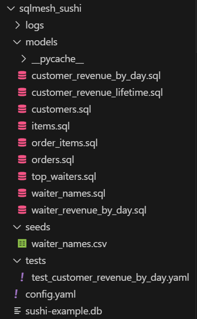
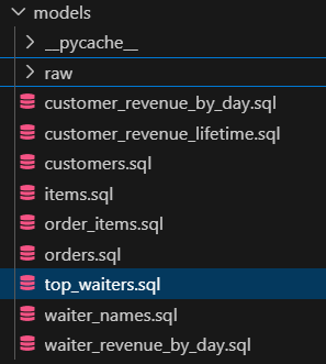
You will see your SQLMesh project scaffolded in your File Explorer window. 

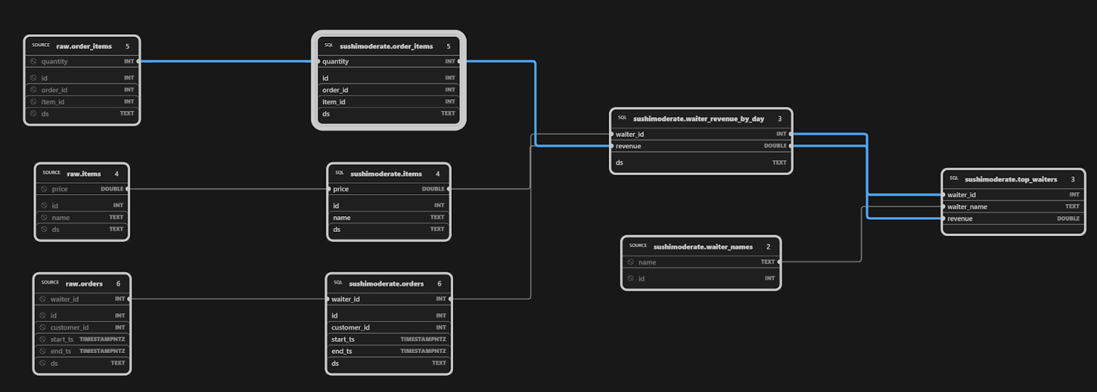
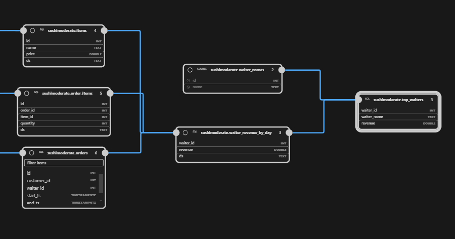
The SQLMesh extension provides a lineage tab, rendering, completion, and diagnostics. Click on model, top_waiters.sql, to see its column-level lineage:

Review the Configuration

Your config.yaml identifies DuckDB as our local database:

gateways:
    local:
        connection:
            type: duckdb
            database: sushi-example.db

default_gateway: local

model_defaults:
    dialect: duckdb

What’s in the project?

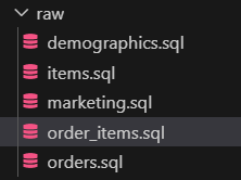
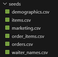
• models/raw: seed-backed raw tables for the sushi dataset (orders, order items, items, customers). These load the seed CSVs.

• models/…: staging and incremental SQL models that transform to clean, join, and aggregate the raw data into analysis-ready facts and small rollups.

• seeds/: CSVs used by the raw Seed models.

• tests/test_customer_revenue_by_day
  
  • A unit test to validate the outputs of the customer_revenue_by_day model based on provided inputs.

Let’s test your configuration. If you don’t receive any errors, then you are good to go!

sqlmesh info

What we need to add:

• To predictively cluster customers into a hierarchy of lifetime value, we first need to calculate and materialize the data set. We will add a customer_lifetime_value model to roll the transactional facts up to a per-customer table with a basic lifetime_value calculation, with historical_revenue, and active_months columns. This is the dataset that our clustering model will be based on.
  
  
• We will add a customer_segments Python model to do our segmentation and materialize the dataframe that marketing can access for their segmentation campaign. This model will perform the clustering and assign marketing-friendly segment labels. 

Why add customer_lifetime_value.sql model before customer_segments.py?

• SQL should do the set-based heavy lifting (joins, filters, date math) to produce a small, tidy, per-customer table. Python should do the algorithmic work (k-means and labeling). Splitting responsibilities keeps both sides simple and testable.
  
  
• Lineage and environments: when customer_lifetime_value exists, the Python model can resolve it via context.resolve_table, so dev and prod read the right physical table automatically, and the dependency shows up in lineage.
  
  
• Performance and stability: pushing the wide scans and aggregations into SQL keeps the Python step light. The clustering model then reads a compact DataFrame with well-typed columns and a stable schema, which makes results reproducible and easier to validate.
  

Add the customer_lifetime_value SQL model

MODEL (
  name sushimoderate.customer_lifetime_value,
  kind FULL,
  owner analytics,
  grain customer_id,
  audits (
    unique_values(columns := customer_id),
    not_null(columns := (customer_id, lifetime_value))
  )
);

WITH per_customer AS (
  SELECT
    crl.customer_id::INT AS customer_id,
    MIN(CAST(crl.ds AS DATE)) AS first_order_date,
    MAX(CAST(crl.ds AS DATE)) AS last_order_date,
    COUNT(DISTINCT DATE_TRUNC('month', CAST(crl.ds AS DATE))) AS active_months,
    -- cumulative series: take the final cumulative revenue for each customer
    MAX(crl.revenue)::DOUBLE AS historical_revenue
  FROM sushimoderate.customer_revenue_lifetime AS crl
  GROUP BY crl.customer_id
)
SELECT
  pc.customer_id,
  pc.first_order_date,
  pc.active_months,
  pc.historical_revenue,
  CASE
    WHEN pc.active_months >= 6 THEN pc.historical_revenue * 2.5
    WHEN pc.active_months >= 3 THEN pc.historical_revenue * 2.0
    ELSE pc.historical_revenue * 1.5
  END AS lifetime_value
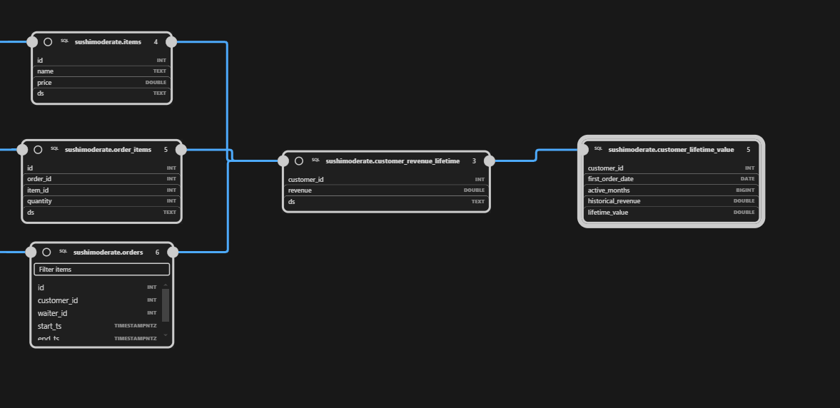
FROM per_customer AS pc;

Even before we run any additional commands, the SQLMesh extension has already picked up this model and added it to our lineage graph:

Let’s create a test to validate the accuracy of the table going forward.

# tests/test_customer_lifetime_value.yaml
test_customer_lifetime_value:
  model: sushimoderate.customer_lifetime_value
  inputs:
    sushimoderate.customer_revenue_lifetime:
      # cumulative series for a single customer across 3 months
      - {customer_id: 1, ds: 2024-01-01, revenue: 100}
      - {customer_id: 1, ds: 2024-02-01, revenue: 250}
      - {customer_id: 1, ds: 2024-03-01, revenue: 450}
  outputs:
    query:
      - customer_id: 1
        first_order_date: 2024-01-01
        active_months: 3
        historical_revenue: 450.0
        lifetime_value: 900.0

Now add this model to the dev environment and backfill the models:

sqlmesh plan dev
.
======================================================================
Successfully Ran 1 tests against duckdb in 0.13 seconds.
----------------------------------------------------------------------

`dev` environment will be initialized

Models:
└── Added:
    ├── raw__dev.demographics
    ├── .... 13 more ....
    └── sushimoderate__dev.waiter_revenue_by_day
Models needing backfill:
├── raw__dev.demographics: [full refresh]
├── .... 13 more ....
└── sushimoderate__dev.waiter_revenue_by_day: [2023-01-01 - 2025-08-10]
Apply - Backfill Tables [y/n]: y

Executing model batches ━━━━━━━━━━━━━━━━━━━━━━━━━━━━━━━━━━━━━━━━ 100.0% • 694/694 • 0:00:30                                                                                                     

✔ Model batches executed

Updating virtual layer  ━━━━━━━━━━━━━━━━━━━━━━━━━━━━━━━━━━━━━━━━ 100.0% • 15/15 • 0:00:00

✔ Virtual layer updated

Let’s break down what this model is doing:

• The model configuration declares a full-refresh table named sushimoderate.customer_lifetime_value with owner analytics and grain customer_id. Two built-in audits are enabled: unique_values on customer_id (no duplicate customers) and not_null on customer_id and lifetime_value.
  
  
• Reads from sushimoderate.customer_revenue_lifetime, which contains a cumulative revenue series per customer across days.
  
  
• CTE per_customer. Aggregates to one row per customer:
  
  
  
  • customer_id cast to INT,
    
    
  • first_order_date and last_order_date from min/max ds,
    
    
  • active_months via count distinct month(ds),
    
    
  • historical_revenue as the max of the cumulative revenue series (final total). Types are normalized (e.g., DOUBLE) during aggregation.
    
    
• The final SELECT identifies customer_id, first_order_date, active_months, historical_revenue, and computes lifetime_value with a tiered multiplier based on tenure:
  
  
  
  • active_months ≥ 6 → 2.5× historical_revenue
    
    
  • active_months ≥ 3 → 2.0×
    
    
  • otherwise → 1.5×
    This produces a clean, per-customer table our downstream Python model can consume.

Let’s review the table output:

sqlmesh fetchdf "select * from sushimoderate__dev.customer_lifetime_value limit 5"

‍Let’s push this new model to production:

sqlmesh plan

======================================================================
Successfully Ran 1 tests against duckdb in 0.05 seconds.
----------------------------------------------------------------------

`prod` environment will be initialized

Models:
└── Added:
    ├── raw.demographics
    ├── .... 13 more ....
    └── sushimoderate.waiter_revenue_by_day
Apply - Virtual Update [y/n]: y

SKIP: No physical layer updates to perform

SKIP: No model batches to execute

Updating virtual layer  ━━━━━━━━━━━━━━━━━━━━━━━━━━━━━━━━━━━━━━━━ 100.0% • 15/15 • 0:00:00

✔ Virtual layer updated

Add the customer_segments Python model

For our clustering model, we’ll read our new sushimoderate.customer_lifetime_value, engineer features, pick k by silhouette over a small range, and label clusters by average LTV.

Create models/customer_segments.py:

# File: models/customer_segments.py
from __future__ import annotations

from typing import Any, Dict, List, Iterator

import numpy as np
import pandas as pd
from sqlmesh import ExecutionContext, model
from sqlmesh.core.model.kind import ModelKindName


@model(
    "sushimoderate.customer_segments",
    # Full refresh each run so the whole population is rescored.
    kind=dict(name=ModelKindName.FULL),
    owner="analytics",
    grains=["customer_id"],
       columns={
        "customer_id": "int",
        "lifetime_value": "double",
        "historical_revenue": "double",
        "active_months": "bigint",
        "value_rate": "double",
        "cluster": "int",
        "segment": "text",
        "silhouette": "double",
    },
)
def execute(context: ExecutionContext, **kwargs: Any) -> Iterator[pd.DataFrame]:
    """
    Segment customers using k-means with k-means++ init and silhouette-based k selection.

    Source model: sushimoderate.customer_lifetime_value
    Features: log1p(lifetime_value), log1p(historical_revenue), log1p(value_rate), active_months
    Weights: lifetime_value emphasized so 'Top' aligns with monetary value.
    """

    # Resolve the upstream table name for the current environment and register dependency.
    clv_table = context.resolve_table("sushimoderate.customer_lifetime_value")

    src_sql = f"""
        SELECT
            customer_id,
            lifetime_value,
            historical_revenue,
            active_months
        FROM {clv_table}
    """
    df = context.fetchdf(src_sql)

    # If upstream has no rows, yield nothing (SQLMesh treats this as an empty result with the declared schema).
    if df is None or df.empty:
        return

    # Basic typing / cleaning
    df["customer_id"] = df["customer_id"].astype(int)
    df["lifetime_value"] = df["lifetime_value"].astype(float)
    df["historical_revenue"] = df["historical_revenue"].astype(float)
    df["active_months"] = df["active_months"].fillna(0).astype(int)

    # Feature engineering
    df["value_rate"] = df["historical_revenue"] / np.maximum(df["active_months"], 1)

    # Build feature matrix: log1p-transform skewed monetary features, keep active_months as-is
    feats = np.column_stack(
        [
            np.log1p(df["lifetime_value"].to_numpy()),
            np.log1p(df["historical_revenue"].to_numpy()),
            np.log1p(df["value_rate"].to_numpy()),
            df["active_months"].to_numpy().astype(float),
        ]
    )

    # Standardize
    mu = feats.mean(axis=0)
    sigma = feats.std(axis=0)
    sigma[sigma == 0.0] = 1.0
    X = (feats - mu) / sigma

    # Emphasize monetary value dimensions
    weights = np.array([2.0, 1.0, 1.2, 0.6])  # lifetime_value gets most weight
    Xw = X * weights

    rng = np.random.default_rng(42)

    def kmeans_pp_init(x: np.ndarray, k: int) -> np.ndarray:
        n = x.shape[0]
        centers = np.empty((k, x.shape[1]), dtype=float)
        # First center
        idx = rng.integers(0, n)
        centers[0] = x[idx]
        # Subsequent centers
        closest_sq = ((x - centers[0]) ** 2).sum(axis=1)
        for j in range(1, k):
            probs = closest_sq / closest_sq.sum()
            idx = rng.choice(n, p=probs)
            centers[j] = x[idx]
            d2 = ((x - centers[j]) ** 2).sum(axis=1)
            closest_sq = np.minimum(closest_sq, d2)
        return centers

    def kmeans_fit(x: np.ndarray, k: int, n_init: int = 8, max_iter: int = 200, tol: float = 1e-6):
        best_inertia = np.inf
        best_labels = None
        best_centers = None
        for _ in range(n_init):
            centers = kmeans_pp_init(x, k)
            labels = np.zeros(x.shape[0], dtype=int)
            for _ in range(max_iter):
                # Assign
                d2 = ((x[:, None, :] - centers[None, :, :]) ** 2).sum(axis=2)
                new_labels = d2.argmin(axis=1)
                # Update
                new_centers = np.stack(
                    [x[new_labels == j].mean(axis=0) if np.any(new_labels == j) else centers[j] for j in range(k)]
                )
                if np.linalg.norm(new_centers - centers) < tol:
                    labels = new_labels
                    centers = new_centers
                    break
                labels = new_labels
                centers = new_centers
            inertia = ((x - centers[labels]) ** 2).sum()
            if inertia < best_inertia:
                best_inertia = inertia
                best_labels = labels
                best_centers = centers
        return best_labels, best_centers, float(best_inertia)

    def silhouette_scores(x: np.ndarray, labels: np.ndarray) -> np.ndarray:
        # Pairwise Euclidean distances (OK for small N like this example)
        n = x.shape[0]
        sum_sq = (x ** 2).sum(axis=1, keepdims=True)
        d2 = sum_sq + sum_sq.T - 2 * (x @ x.T)
        d2 = np.maximum(d2, 0.0)
        d = np.sqrt(d2)

        s = np.zeros(n, dtype=float)
        for i in range(n):
            same = labels == labels[i]
            other = ~same
            # a: mean distance to same-cluster points (exclude self)
            if same.sum() > 1:
                a = d[i, same].sum() / (same.sum() - 1)
            else:
                a = 0.0
            # b: minimal mean distance to points in other clusters
            b = np.inf
            for cl in np.unique(labels[other]):
                mask = labels == cl
                b = min(b, d[i, mask].mean())
            s[i] = 0.0 if max(a, b) == 0 else (b - a) / max(a, b)
        return s

    # Choose k by silhouette in [3..6], bounded by n
    n = Xw.shape[0]
    k_candidates = [k for k in range(3, 7) if k <= n]
    if not k_candidates:
        # Fallback: single cluster
        df["cluster"] = 0
        df["segment"] = "Top"
        df["silhouette"] = 0.0
    else:
        best = None
        best_score = -np.inf
        for k in k_candidates:
            labels, centers, _ = kmeans_fit(Xw, k=k)
            s = silhouette_scores(Xw, labels)
            score = float(np.nan_to_num(s).mean())
            if score > best_score:
                best = (k, labels, s)
                best_score = score

        k, labels, s = best
        df["cluster"] = labels.astype(int)
        df["silhouette"] = s.astype(float)

        # Label clusters by ascending mean lifetime_value
        means = df.groupby("cluster")["lifetime_value"].mean().sort_values()
        order = list(means.index)  # ascending by LTV
        names_by_k: Dict[int, List[str]] = {
            3: ["Low", "Mid", "Top"],
            4: ["Low", "Mid", "High", "Top"],
            5: ["Very Low", "Low", "Mid", "High", "Top"],
            6: ["Very Low", "Low", "Mid", "High", "Very High", "Top"],
        }
        labels_for_k = names_by_k.get(k, ["Low", "Mid", "High", "Top"][:k])
        name_map = {cl: labels_for_k[i] for i, cl in enumerate(order)}
        df["segment"] = df["cluster"].map(name_map).astype(str)

    out = df[
        [
            "customer_id",
            "lifetime_value",
            "historical_revenue",
            "active_months",
            "value_rate",
            "cluster",
            "segment",
            "silhouette",
        ]
    ].copy()

    # Ensure declared types
    out["customer_id"] = out["customer_id"].astype(int)
    out["active_months"] = out["active_months"].astype(int)
    out["cluster"] = out["cluster"].astype(int)
    out["lifetime_value"] = out["lifetime_value"].astype(float)
    out["historical_revenue"] = out["historical_revenue"].astype(float)
    out["value_rate"] = out["value_rate"].astype(float)
    out["silhouette"] = out["silhouette"].astype(float)
    out["segment"] = out["segment"].astype(str)

    # Yield the final frame (chunked-output friendly). If no rows upstream, we yielded nothing above.
    yield out

Let’s break down the customer_segments.py model components:

1. Model metadata
   The @model decorator makes this a SQLMesh model. We give it a name (sushimoderate.customer_segments), set kind to FULL (rebuild every run—right for clustering), declare the grain (customer_id), list its upstream dependency (sushimoderate.customer_lifetime_value), and define the output columns and types so SQLMesh can create the table.
   
   
2. Execution contract
   SQLMesh calls execute(context, …). The function yields a DataFrame (not returns) so we can stream results and, if there’s no data upstream, yield nothing. That empty case is required for Python models.
   
   
3. Reading upstream safely
   context.resolve_table(...) gets the environment‑aware table name for customer_lifetime_value; context.fetchdf(...) runs a SELECT and returns a pandas DataFrame. This keeps dev/prod isolation correct and captures modellineage.
   
   
4. Type hygiene
   We enforce types such as customer_id to int; monetary fields to float; active_months to int (after filling nulls). This aligns the DataFrame with the declared schema and prevents type surprises later.
   
   
5. Quick feature engineering
   We add value_rate = historical_revenue / max(active_months, 1). It’s a simple velocity feature that complements lifetime_value and total spend.
   
   
6. Make features cluster‑friendly
   Build a matrix and standardize to zero‑mean/unit‑variance; then apply weights [2.0, 1.0, 1.2, 0.6] to emphasize customer value.
   
   
7. Fit k‑means
   Initialize centers with k‑means++ for better starts, run k‑means multiple times (n_init), and keep the best solution by inertia. Seeded RNG makes results reproducible.
   
   
8. Let the data choose k
   Try k in [3..6] (bounded by row count). For each k, compute silhouettes and pick the k with the highest mean silhouette. If too few rows for k ≥ 3, default to one cluster so the model still emits a valid table.
   
   
9. Name segments to align with Marketing requirements
   Assign cluster labels, then sort clusters by mean lifetime_value and map them to ordered names (e.g., Very Low → Low → Mid → High → Top). This keeps labels stable and intuitive even if raw cluster IDs shift.
   
   
10. Emit a clean table
    Select exactly the declared columns in order, re‑cast types defensively, and yield the final DataFrame. SQLMesh writes it as sushimoderate.customer_segments (or the dev‑suffixed schema in a dev environment), and the lineage shows it downstream of customer_lifetime_value.
    
    

Let’s add our Python model to our dev environment, and review the output:

sqlmesh plan dev
.
======================================================================
Successfully Ran 1 tests against duckdb in 0.05 seconds.
----------------------------------------------------------------------

Differences from the `dev` environment:

Requirements:
    + numpy==2.3.2
Models:
└── Added:
    └── sushimoderate__dev.customer_segments
Models needing backfill:
└── sushimoderate__dev.customer_segments: [full refresh]
Apply - Backfill Tables [y/n]: y

Updating physical layer ━━━━━━━━━━━━━━━━━━━━━━━━━━━━━━━━━━━━━━━━ 100.0% • 1/1 • 0:00:00

✔ Physical layer updated

[1/1] sushimoderate__dev.customer_segments   [full refresh]   0.06s   
Executing model batches ━━━━━━━━━━━━━━━━━━━━━━━━━━━━━━━━━━━━━━━━ 100.0% • 1/1 • 0:00:00

✔ Model batches executed

Updating virtual layer  ━━━━━━━━━━━━━━━━━━━━━━━━━━━━━━━━━━━━━━━━ 100.0% • 16/16 • 0:00:00

✔ Virtual layer updated

Let’s explore the output:

sqlmesh fetchdf "select * from sushimoderate__dev.customer_segments limit 5"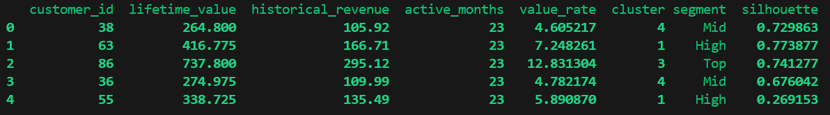

sqlmesh fetchdf "select segment, count(customer_id), avg(silhouette) from sushimoderate__dev.customer_segments group by segment order by count(customer_id) desc"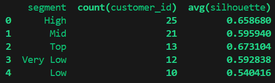

Now, let’s promote the Python model to production:

sqlmesh plan

======================================================================
Successfully Ran 1 tests against duckdb in 0.05 seconds.
----------------------------------------------------------------------

Differences from the `prod` environment:

Requirements:
    + numpy==2.3.2
Models:
└── Added:
    └── sushimoderate.customer_segments
Apply - Virtual Update [y/n]: y

SKIP: No physical layer updates to perform

SKIP: No model batches to execute

Updating virtual layer  ━━━━━━━━━━━━━━━━━━━━━━━━━━━━━━━━━━━━━━━━ 100.0% • 1/1 • 0:00:00

✔ Virtual layer updated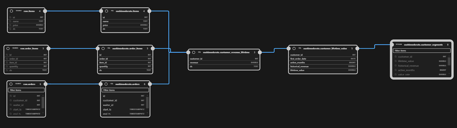

How Marketing Can Use the Output

Marketing now has a clean table with customer_id, metrics, cluster, segment, and a quality metric silhouette that they can pull into their CRM system. Campaign managers can pull Top and High segments for promotions, or analyze spend by segment. Data engineering keeps the same SQLMesh advantages: deterministic plans, environment isolation, reproducible promotions, and an interactive lineage graph that shows exactly where the Python model sits.

Conclusion

In this tutorial, we demonstrated the power and flexibility of SQLMesh Python models. We started from a conventional SQL-based data pipeline, identified a use case (customer segmentation via k-means for a marketing campaign) that benefits from Python, and seamlessly plugged a new Python model into the project. 

Key takeaways:

• SQLMesh allows data engineers the flexibility to break out of SQL when needed and leverage Python’s ecosystem, all while maintaining versioned, testable, and schedulable pipelines. Complex analytics and machine learning can live alongside traditional SQL transformations in one framework.
  
  
• The SQLMesh VS Code extension accelerates development. We used it to understand our project and worked without switching contexts.
  
  
• When creating Python models, remember to declare your output schema and any dependencies. This enables SQLMesh to handle table creation and upstream scheduling correctly. Be mindful of data sizes (chunk output or use Spark if necessary for big data).
  
  
• We employed k-means within a pipeline as a POC. With SQLMesh, complex models can be treated as first-class citizens and benefit from the same dev/prod environment isolation, tests, and review process that makes SQLMesh great!

Happy Engineering!

{{cta-talk}}

{{banner-slack}}